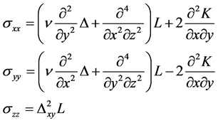
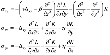
<?xml version="1.0" encoding="UTF-8"?><!DOCTYPE article  PUBLIC "-//NLM//DTD Journal Publishing DTD v3.0 20080202//EN" "http://dtd.nlm.nih.gov/publishing/3.0/journalpublishing3.dtd"><article xmlns:mml="http://www.w3.org/1998/Math/MathML" xmlns:xlink="http://www.w3.org/1999/xlink" dtd-version="3.0" xml:lang="en" article-type="research article"><front><journal-meta><journal-id journal-id-type="publisher-id">OALibJ</journal-id><journal-title-group><journal-title>Open Access Library Journal</journal-title></journal-title-group><issn pub-type="epub">2333-9705</issn><publisher><publisher-name>Scientific Research Publishing</publisher-name></publisher></journal-meta><article-meta><article-id pub-id-type="doi">10.4236/oalib.1101670</article-id><article-id pub-id-type="publisher-id">OALibJ-68484</article-id><article-categories><subj-group subj-group-type="heading"><subject>Articles</subject></subj-group><subj-group subj-group-type="Discipline-v2"><subject>Biomedical&amp;Life Sciences</subject><subject> Business&amp;Economics</subject><subject> Chemistry&amp;Materials Science</subject><subject> Computer Science&amp;Communications</subject><subject> Earth&amp;Environmental Sciences</subject><subject> Engineering</subject><subject> Medicine&amp;Healthcare</subject><subject> Physics&amp;Mathematics</subject><subject> Social Sciences&amp;Humanities</subject></subj-group></article-categories><title-group><article-title>
 
 
  Unidimensional Inhomogeneous Isotropic Elastic Half-Space
 
</article-title></title-group><contrib-group><contrib contrib-type="author" xlink:type="simple"><name name-style="western"><surname>Igor</surname><given-names>Petrovich Dobrovolsky</given-names></name><xref ref-type="aff" rid="aff1"><sub>1</sub></xref><xref ref-type="corresp" rid="cor1"><sup>*</sup></xref></contrib></contrib-group><aff id="aff1"><label>1</label><addr-line>Institute of Physics of the Earth, Russian Academy of Sciences, Moscow, Russia</addr-line></aff><author-notes><corresp id="cor1">* E-mail:<email>dipedip@gmail.com</email></corresp></author-notes><pub-date pub-type="epub"><day>31</day><month>07</month><year>2015</year></pub-date><volume>02</volume><issue>07</issue><fpage>1</fpage><lpage>6</lpage><history><date date-type="received"><day>15</day>	<month>June</month>	<year>2015</year></date><date date-type="rev-recd"><day>accepted</day>	<month>1</month>	<year>July</year>	</date><date date-type="accepted"><day>8</day>	<month>July</month>	<year>2015</year></date></history><permissions><copyright-statement>&#169; Copyright  2014 by authors and Scientific Research Publishing Inc. </copyright-statement><copyright-year>2014</copyright-year><license><license-p>This work is licensed under the Creative Commons Attribution International License (CC BY). http://creativecommons.org/licenses/by/4.0/</license-p></license></permissions><abstract><p>


   The homogeneous system of the equations of the linear theory of elasticity for the isotropic environment with one-dimensional continuous heterogeneity is considered. Bidimensional transformation Fourier is applied and the problem for images is led to the ordinary differential equations. Generally, the differential equations are transformed in integro-differential and the algorithm of such transformation is resulted. Solutions of specific problems are resulted. 
  
 
</p></abstract><kwd-group><kwd>Continuous Heterogeneity</kwd><kwd> The Integro-Differential Equation</kwd><kwd> Bidimensional Fourier’s  Transformation</kwd></kwd-group></article-meta></front><body><sec id="s1"><title>1. Introduction</title><p>The elastic half-space is considered inhomogeneous along depth. Such problems were investigated in many works (for example, [<xref ref-type="bibr" rid="scirp.68484-ref1">1</xref>] - [<xref ref-type="bibr" rid="scirp.68484-ref3">3</xref>] ). The detailed review is not the purpose of this paper, but the technique applied in the paper does not meet in publications. Let’s note that problems for an elastic half-space are especially important in a science about the Earth as the Earth’s crust is usually modelled by a half-space.</p><p>Research is made with application of bidimensional transformation Fourier which leads to the ordinary differential equations. The method of transition to integral equations [<xref ref-type="bibr" rid="scirp.68484-ref4">4</xref>] is applied to their solution. Such technique expands a circle of problems for which it is possible to find the satisfactory approached solution. The concrete example is resulted.</p></sec><sec id="s2"><title>2. Statement of the Problem</title><p>In cartesian coordinates (x, y, z) it is considered isotropic inhomogeneous on z an elastic half-space z ≥ 0 with the shear modulus μ(z) and coefficient of Poisson ν(z). In this case the homogeneous system of the equations of the theory of elasticity in displacements (u, v, w) looks like</p><disp-formula id="scirp.68484-formula40"><label>(2.1)</label><graphic position="anchor" xlink:href="http://html.scirp.org/file/68484x5.png"  xlink:type="simple"/></disp-formula><p>where <inline-formula><inline-graphic xlink:href="http://html.scirp.org/file/68484x6.png" xlink:type="simple"/></inline-formula> is a volume strain, ω = 1 − 2ν, Δ is Laplace operator on three variables, the comma in an inferior index means a derivative on corresponding variable.</p><p>In [<xref ref-type="bibr" rid="scirp.68484-ref5">5</xref>] it is shown, that the system (2.1) is equivalent to system for two functions</p><disp-formula id="scirp.68484-formula41"><label>(2.2)</label><graphic position="anchor" xlink:href="http://html.scirp.org/file/68484x7.png"  xlink:type="simple"/></disp-formula><p>where η = d(lnμ)/dz. β = 1 − ν, Δ<sub>xy</sub> is Laplace operator on two variables.</p><p>Displacements are expressed by formulas</p><disp-formula id="scirp.68484-formula42"><label>(2.3)</label><graphic position="anchor" xlink:href="http://html.scirp.org/file/68484x8.png"  xlink:type="simple"/></disp-formula><p>and stresses are</p><p><img src="http://html.scirp.org/file/68484x9.png" /> <img src="http://html.scirp.org/file/68484x10.png" />. (2.4)</p><p>Formulas (2.1)-(2.4) are received in the monograph [<xref ref-type="bibr" rid="scirp.68484-ref5">5</xref>] . Here it have undergone to some transformations.</p><p>To a half-space (or a lay) we shall apply bidimensional transformation Fourier in the form of</p><disp-formula id="scirp.68484-formula43"><label>(2.5)</label><graphic position="anchor" xlink:href="http://html.scirp.org/file/68484x11.png"  xlink:type="simple"/></disp-formula><p>where i is imaginary unit.</p><p>Then the basic operators will be transformed by formulas</p><disp-formula id="scirp.68484-formula44"><label>. (2.6)</label><graphic position="anchor" xlink:href="http://html.scirp.org/file/68484x12.png"  xlink:type="simple"/></disp-formula><p>For functions <inline-formula><inline-graphic xlink:href="http://html.scirp.org/file/68484x13.png" xlink:type="simple"/></inline-formula> and <inline-formula><inline-graphic xlink:href="http://html.scirp.org/file/68484x14.png" xlink:type="simple"/></inline-formula> the system (2.2) gets an aspect</p><disp-formula id="scirp.68484-formula45"><label>. (2.7)</label><graphic position="anchor" xlink:href="http://html.scirp.org/file/68484x15.png"  xlink:type="simple"/></disp-formula><p>Transformations of stresses on a plane z = const are</p><disp-formula id="scirp.68484-formula46"><label>. (2.8)</label><graphic position="anchor" xlink:href="http://html.scirp.org/file/68484x16.png"  xlink:type="simple"/></disp-formula><p>The problem is reduced to a solution of the ordinary linear differential equations for functions <inline-formula><inline-graphic xlink:href="http://html.scirp.org/file/68484x17.png" xlink:type="simple"/></inline-formula> and <inline-formula><inline-graphic xlink:href="http://html.scirp.org/file/68484x18.png" xlink:type="simple"/></inline-formula> with corresponding boundary conditions. The reversion of transformation of Fourier (calculation of definite integrals) does not cause difficulties for modern mathematical programs.</p></sec><sec id="s3"><title>3. The Equation for <inline-formula><inline-graphic xlink:href="http://html.scirp.org/file/68484x19.png" xlink:type="simple"/></inline-formula></title><p>The first equation from (2.7) we will write down in a kind</p><disp-formula id="scirp.68484-formula47"><label>. (3.1)</label><graphic position="anchor" xlink:href="http://html.scirp.org/file/68484x20.png"  xlink:type="simple"/></disp-formula><p>One of ways of search of the approached the general solution of the Equation (3.1) for any smooth function μ(z) is transition to the integro-differential equation on algorithm [<xref ref-type="bibr" rid="scirp.68484-ref4">4</xref>] . In so doing an operator <inline-formula><inline-graphic xlink:href="http://html.scirp.org/file/68484x21.png" xlink:type="simple"/></inline-formula> is chosen by the basic operator, because for a homogeneous environment (μ = const) the Equation (3.1) has form<inline-formula><inline-graphic xlink:href="http://html.scirp.org/file/68484x21.png" xlink:type="simple"/></inline-formula><inline-formula><inline-graphic xlink:href="http://html.scirp.org/file/68484x22.png" xlink:type="simple"/></inline-formula>.</p><p>For a finite segment we use the general solution of the inhomogeneous equation<inline-formula><inline-graphic xlink:href="http://html.scirp.org/file/68484x23.png" xlink:type="simple"/></inline-formula>. The homogeneous equation <inline-formula><inline-graphic xlink:href="http://html.scirp.org/file/68484x23.png" xlink:type="simple"/></inline-formula><inline-formula><inline-graphic xlink:href="http://html.scirp.org/file/68484x24.png" xlink:type="simple"/></inline-formula> has a Green function limited on infinity [<xref ref-type="bibr" rid="scirp.68484-ref6">6</xref>]</p><disp-formula id="scirp.68484-formula48"><label>. (3.2)</label><graphic position="anchor" xlink:href="http://html.scirp.org/file/68484x25.png"  xlink:type="simple"/></disp-formula><p>It allows to construct the equation for a semi-infinite segment.</p><p>As a result we come to two integro-differential equations of the II kind:</p><p>for layer</p><disp-formula id="scirp.68484-formula49"><label>(3.3)</label><graphic position="anchor" xlink:href="http://html.scirp.org/file/68484x26.png"  xlink:type="simple"/></disp-formula><p>and for a half-space</p><disp-formula id="scirp.68484-formula50"><label>. (3.4)</label><graphic position="anchor" xlink:href="http://html.scirp.org/file/68484x27.png"  xlink:type="simple"/></disp-formula><p>By integration by parts (3.3) and (3.4) will be transformed to integral equations</p><disp-formula id="scirp.68484-formula51"><label>, (3.5)</label><graphic position="anchor" xlink:href="http://html.scirp.org/file/68484x28.png"  xlink:type="simple"/></disp-formula><disp-formula id="scirp.68484-formula52"><label>. (3.6)</label><graphic position="anchor" xlink:href="http://html.scirp.org/file/68484x29.png"  xlink:type="simple"/></disp-formula><p>If for the equation <inline-formula><inline-graphic xlink:href="http://html.scirp.org/file/68484x30.png" xlink:type="simple"/></inline-formula> it is possible to construct a Green function for the chosen boundary conditions, then for Equation (3.1) corresponding integral equations are possible to construct for these conditions with its help. Equation (3.4) is an example.</p></sec><sec id="s4"><title>4. The Equation for <inline-formula><inline-graphic xlink:href="http://html.scirp.org/file/68484x31.png" xlink:type="simple"/></inline-formula></title><p>Let’s note the second equation of system (2.7) in the form</p><disp-formula id="scirp.68484-formula53"><label>, (4.1)</label><graphic position="anchor" xlink:href="http://html.scirp.org/file/68484x32.png"  xlink:type="simple"/></disp-formula><p>where<inline-formula><inline-graphic xlink:href="http://html.scirp.org/file/68484x33.png" xlink:type="simple"/></inline-formula>.</p><p>If to apply to the Equation (4.1) operator, inverse to<inline-formula><inline-graphic xlink:href="http://html.scirp.org/file/68484x34.png" xlink:type="simple"/></inline-formula>, (as it is made in the previous section) then we receive two integral equations:</p><p>For a layer</p><disp-formula id="scirp.68484-formula54"><label>(4.2)</label><graphic position="anchor" xlink:href="http://html.scirp.org/file/68484x35.png"  xlink:type="simple"/></disp-formula><p>And for a half-space</p><disp-formula id="scirp.68484-formula55"><label>. (4.3)</label><graphic position="anchor" xlink:href="http://html.scirp.org/file/68484x36.png"  xlink:type="simple"/></disp-formula><p>At μ = 1/(az+b) function Q(z) = 0 and Formulas (4.2) and (4.3) give the exact general solution of the equation (4.1).</p></sec><sec id="s5"><title>5. Solution of the Specific Problem</title><p>We shall consider a problem about unit force on a surface of a half-space z ≥ 0 in the origin of coordinates. Apparently from system (2.8), in this case (and, in general, for problems with axial symmetry) it is possible to put <inline-formula><inline-graphic xlink:href="http://html.scirp.org/file/68484x37.png" xlink:type="simple"/></inline-formula> = 0. For function <inline-formula><inline-graphic xlink:href="http://html.scirp.org/file/68484x37.png" xlink:type="simple"/></inline-formula><inline-formula><inline-graphic xlink:href="http://html.scirp.org/file/68484x38.png" xlink:type="simple"/></inline-formula> boundary conditions receive the form</p><disp-formula id="scirp.68484-formula56"><label>. (5.1)</label><graphic position="anchor" xlink:href="http://html.scirp.org/file/68484x39.png"  xlink:type="simple"/></disp-formula><p>Let’s put</p><disp-formula id="scirp.68484-formula57"><label>. (5.2)</label><graphic position="anchor" xlink:href="http://html.scirp.org/file/68484x40.png"  xlink:type="simple"/></disp-formula><p>Then the Equation (4.1) has the solution limited on infinity</p><disp-formula id="scirp.68484-formula58"><label>. (5.3)</label><graphic position="anchor" xlink:href="http://html.scirp.org/file/68484x41.png"  xlink:type="simple"/></disp-formula><p>Here C<sub>1</sub> and C<sub>2</sub> are arbitrary constants, ζ = ρ(1 + z), Ψ(α, β; x) is degenerate hypergeometric function of 2-nd sort or Kummer’s function of 2-nd kind. In computer program Maple this function is designated as Kummer U (α, β, z) and it has integral representation</p><disp-formula id="scirp.68484-formula59"><label>(5.4)</label><graphic position="anchor" xlink:href="http://html.scirp.org/file/68484x42.png"  xlink:type="simple"/></disp-formula><p>where Γ(a) is the gamma-function.</p><p>It is simple to receive the solution of the problem (5.1)-(5.3) in Fourier transformations, but to carry out the inverse Fourier transform through known functions is not receive. However it is possible to approximate special functions by combinations of elementary functions. Approximation can be made with a demanded exactitude and simplifies the further calculations. In particular for (5.3) we have</p><disp-formula id="scirp.68484-formula60"><label>. (5.5)</label><graphic position="anchor" xlink:href="http://html.scirp.org/file/68484x43.png"  xlink:type="simple"/></disp-formula><p>The error of this approximation does not exceed 0.5 %.</p><p>Level lines of stress σ<sub>zz</sub> are shown on <xref ref-type="fig" rid="fig1">Figure 1</xref>. The narrow layer at the half-space surface is empty because it is necessary to show it in larger scale though qualitative behaviour of level lines in this layer to present simply. Existence of a zone of small tensile stresses is the basic singularity of this graph. In a homogeneous half-space</p><fig id="fig1"  position="float"><label><xref ref-type="fig" rid="fig1">Figure 1</xref></label><caption><title> Level lines of stress the exact σ<sub>zz</sub> solution. Black area is the zone of positive values</title></caption><graphic mimetype="image"   position="float"  xlink:type="simple"  xlink:href="http://html.scirp.org/file/68484x44.png"/></fig><p>(the Boussinesq’s problem) such zone does not arise.</p><p>It is interesting to compare the received solution to the approximate solution. As the approximate solution we take the zero approximation for the Equation (4.3). Such solution turns out at Q = 0 and it has the form</p><disp-formula id="scirp.68484-formula61"><label>. (5.6)</label><graphic position="anchor" xlink:href="http://html.scirp.org/file/68484x45.png"  xlink:type="simple"/></disp-formula><p>Using boundary conditions (5.1) we receive function</p><disp-formula id="scirp.68484-formula62"><label>. (5.7)</label><graphic position="anchor" xlink:href="http://html.scirp.org/file/68484x46.png"  xlink:type="simple"/></disp-formula><p>According to (2.8) transformation of stress σ<sub>zz</sub> gets the form</p><disp-formula id="scirp.68484-formula63"><label>. (5.8)</label><graphic position="anchor" xlink:href="http://html.scirp.org/file/68484x47.png"  xlink:type="simple"/></disp-formula><p>To receive stress σ<sub>zz</sub> it is necessary to calculate integral</p><disp-formula id="scirp.68484-formula64"><label>, (5.9)</label><graphic position="anchor" xlink:href="http://html.scirp.org/file/68484x48.png"  xlink:type="simple"/></disp-formula><p>where <inline-formula><inline-graphic xlink:href="http://html.scirp.org/file/68484x49.png" xlink:type="simple"/></inline-formula> and <inline-formula><inline-graphic xlink:href="http://html.scirp.org/file/68484x49.png" xlink:type="simple"/></inline-formula><inline-formula><inline-graphic xlink:href="http://html.scirp.org/file/68484x50.png" xlink:type="simple"/></inline-formula> is Bessel’s function.</p><p>To calculate (5.9) we will allocate the whole part in the integrand.</p><disp-formula id="scirp.68484-formula65"><label>. (5.10)</label><graphic position="anchor" xlink:href="http://html.scirp.org/file/68484x51.png"  xlink:type="simple"/></disp-formula><p>The integral (5.9) is calculated in elementary functions for first three items from a right part of (5.10). The fourth item leads to the integral</p><disp-formula id="scirp.68484-formula66"><label>, (5.11)</label><graphic position="anchor" xlink:href="http://html.scirp.org/file/68484x52.png"  xlink:type="simple"/></disp-formula><p>which is not expressed in known functions.</p><p>However by means of approximation</p><disp-formula id="scirp.68484-formula67"><label>(5.12)</label><graphic position="anchor" xlink:href="http://html.scirp.org/file/68484x53.png"  xlink:type="simple"/></disp-formula><p>integral (5.11) also can be calculated in elementary functions. This operation is easily supervised because the integral (5.11) can be found in separate points numerically by means of known mathematical programs (for example, Maple or Mathematica).</p><p>Level lines of stress σ<sub>zz</sub> calculated by the described algorithm are shown on <xref ref-type="fig" rid="fig2">Figure 2</xref>. <xref ref-type="fig" rid="fig1">Figure 1</xref> and <xref ref-type="fig" rid="fig2">Figure 2</xref></p><fig id="fig2"  position="float"><label><xref ref-type="fig" rid="fig2">Figure 2</xref></label><caption><title> Level lines of stress σ<sub>zz</sub>. The approximate solution</title></caption><graphic mimetype="image"   position="float"  xlink:type="simple"  xlink:href="http://html.scirp.org/file/68484x54.png"/></fig><p>basically are similar. In the approximate solution the area of small tensile stresses remains but it becomes more extensive and moves further from an origin of coordinates.</p></sec><sec id="s6"><title>6. Conclusion</title><p>Transition to integro-differential (or integral) equations is an effective method of a solution of problems for a half-space (or a layer) with arbitrary heterogeneity. It is very important that the solution of an integral equation gives the approximate general solution of the ordinary differential equation. Procedure of transition to integro- differential (or integral) equations allows constructing such equations for the inhomogeneous differential equations.</p></sec><sec id="s7"><title>Cite this paper</title><p>Igor Petrovich Dobrovolsky, (2015) Unidimensional Inhomogeneous Isotropic Elastic Half-Space. Open Access Library Journal,02,1-6. doi: 10.4236/oalib.1101670</p></sec></body><back><ref-list><title>References</title><ref id="scirp.68484-ref1"><label>1</label><mixed-citation publication-type="other" xlink:type="simple">Gibson, R.E. (1967) Some Results Concerning Displacements and Stresses in a Nonhomogeneous Elastic Half-Space. Geotechnique, 17, 58-67. http://dx.doi.org/10.1680/geot.1967.17.1.58</mixed-citation></ref><ref id="scirp.68484-ref2"><label>2</label><mixed-citation publication-type="other" xlink:type="simple">Brown, P.T. and Gibson, R.E. (1979) Surface Settlement of a Finite Elastic Layer Whose Modulus Increases Linearly with Depth. International Journal for Numerical and Analytical Methods in Geomechanics, 3, 33-47.http://dx.doi.org/10.1002/nag.1610030105</mixed-citation></ref><ref id="scirp.68484-ref3"><label>3</label><mixed-citation publication-type="other" xlink:type="simple">Guler, M.A. and Erdogan, F. (2004) Contact Mechanics of Graded Coatings. International Journal of Solids and Structures, 41, 3865-3889. http://dx.doi.org/10.1016/j.ijsolstr.2004.02.025</mixed-citation></ref><ref id="scirp.68484-ref4"><label>4</label><mixed-citation publication-type="other" xlink:type="simple">Dobrovolsky, I.P. (2014) The Integral Equation, Corresponding to the Ordinary Differential Equation. Open Access Library Journal, 1, e1058. http://dx.doi.org/10.4236/oalib.1101058</mixed-citation></ref><ref id="scirp.68484-ref5"><label>5</label><mixed-citation publication-type="other" xlink:type="simple">Lomakin, V.A. (1976) The Elasticity Theory of Inhomogeneous Solid. The Moscow Univercity, Moscow, 368 p.</mixed-citation></ref><ref id="scirp.68484-ref6"><label>6</label><mixed-citation publication-type="other" xlink:type="simple">Kamke, E. (1959) Differential Gleichungen. L&amp;#246;sungsmetohden und Losungen. Leipzig.</mixed-citation></ref></ref-list></back></article>